| OCR with Keras, TensorFlow, and Deep Learning | 您所在的位置:网站首页 › ocr recognition › OCR with Keras, TensorFlow, and Deep Learning |
OCR with Keras, TensorFlow, and Deep Learning
Click here to download the source code to this post
In this tutorial, you will learn how to train an Optical Character Recognition (OCR) model using Keras, TensorFlow, and Deep Learning. This post is the first in a two-part series on OCR with Keras and TensorFlow: Part 1: Training an OCR model with Keras and TensorFlow (today’s post)Part 2: Basic handwriting recognition with Keras and TensorFlow (next week’s post)For now, we’ll primarily be focusing on how to train a custom Keras/TensorFlow model to recognize alphanumeric characters (i.e., the digits 0-9 and the letters A-Z). Building on today’s post, next week we’ll learn how we can use this model to correctly classify handwritten characters in custom input images. The goal of this two-part series is to obtain a deeper understanding of how deep learning is applied to the classification of handwriting, and more specifically, our goal is to: Become familiar with some well-known, readily available handwriting datasets for both digits and lettersUnderstand how to train deep learning model to recognize handwritten digits and lettersGain experience in applying our custom-trained model to some real-world sample dataUnderstand some of the challenges with real-world noisy data and how we might want to augment our handwriting datasets to improve our model and resultsWe’ll be starting with the fundamentals of using well-known handwriting datasets and training a ResNet deep learning model on these data. To learn how to train an OCR model with Keras, TensorFlow, and deep learning, just keep reading. In the first part of this tutorial, we’ll discuss the steps required to implement and train a custom OCR model with Keras and TensorFlow. We’ll then examine the handwriting datasets that we’ll use to train our model. From there, we’ll implement a couple of helper/utility functions that will aid us in loading our handwriting datasets from disk and then preprocessing them. Given these helper functions, we’ll be able to create our custom OCR training script with Keras and TensorFlow. After training, we’ll review the results of our OCR work. Let’s get started! Our deep learning OCR datasets Figure 1: We are using two datasets for our OCR training with Keras and TensorFlow. On the left, we have the standard MNIST 0-9 dataset. On the right, we have the Kaggle A-Z dataset from Sachin Patel, which is based on the NIST Special Database 19. Figure 1: We are using two datasets for our OCR training with Keras and TensorFlow. On the left, we have the standard MNIST 0-9 dataset. On the right, we have the Kaggle A-Z dataset from Sachin Patel, which is based on the NIST Special Database 19.
In order to train our custom Keras and TensorFlow model, we’ll be utilizing two datasets: The standard MNIST 0-9 dataset by LeCun et al.The Kaggle A-Z dataset by Sachin Patel, based on the NIST Special Database 19The standard MNIST dataset is built into popular deep learning frameworks, including Keras, TensorFlow, PyTorch, etc. A sample of the MNIST 0-9 dataset can be seen in Figure 1 (left). The MNIST dataset will allow us to recognize the digits 0-9. Each of these digits is contained in a 28 x 28 grayscale image. You can read more about MNIST here. But what about the letters A-Z? The standard MNIST dataset doesn’t include examples of the characters A-Z — how are we going to recognize them? The answer is to use the NIST Special Database 19, which includes A-Z characters. This dataset actually covers 62 ASCII hexadecimal characters corresponding to the digits 0-9, capital letters A-Z, and lowercase letters a-z. To make the dataset easier to use, Kaggle user Sachin Patel has released the dataset in an easy to use CSV file. This dataset takes the capital letters A-Z from NIST Special Database 19 and rescales them to be 28 x 28 grayscale pixels to be in the same format as our MNIST data. For this project, we will be using just the Kaggle A-Z dataset, which will make our preprocessing a breeze. A sample of it can be seen in Figure 1 (right). We’ll be implementing methods and utilities that will allow us to: Load both the datasets for MNIST 0-9 digits and Kaggle A-Z letters from diskCombine these datasets together into a single, unified character datasetHandle class label skew/imbalance from having a different number of samples per characterSuccessfully train a Keras and TensorFlow model on the combined datasetPlot the results of the training and visualize the output of the validation data Configuring your OCR development environmentTo configure your system for this tutorial, I first recommend following either of these tutorials: How to install TensorFlow 2.0 on UbuntuHow to install TensorFlow 2.0 on macOSEither tutorial will help you configure your system with all the necessary software for this blog post in a convenient Python virtual environment. Project structureLet’s review the project structure. Once you grab the files from the “Downloads” section of this article, you’ll be presented with the following directory structure: $ tree --dirsfirst --filelimit 10 . ├── pyimagesearch │ ├── az_dataset │ │ ├── __init__.py │ │ └── helpers.py │ ├── models │ │ ├── __init__.py │ │ └── resnet.py │ └── __init__.py ├── a_z_handwritten_data.csv ├── handwriting.model ├── plot.png └── train_ocr_model.py 3 directories, 9 filesOnce we unzip our download, we find that our ocr-keras-tensorflow/ directory contains the following: pyimagesearch module: includes the sub-modules az_dataset for I/O helper files and models for implementing the ResNet deep learning architecture a_z_handwritten_data.csv: contains the Kaggle A-Z dataset handwriting.model: where the deep learning ResNet model is saved plot.png: plots the results of the most recent run of training of ResNet train_ocr_model.py: the main driver file for training our ResNet model and displaying the resultsNow that we have the lay of the land, let’s dig into the I/O helper functions we will use to load our digits and letters. Our OCR dataset helper functionsIn order to train our custom Keras and TensorFlow OCR model, we first need to implement two helper utilities that will allow us to load both the Kaggle A-Z datasets and the MNIST 0-9 digits from disk. These I/O helper functions are appropriately named: load_az_dataset: for the Kaggle A-Z letters load_mnist_dataset: for the MNIST 0-9 digitsThey can be found in the helpers.py file of az_dataset submodules of pyimagesearch. Let’s go ahead and examine this helpers.py file. We will begin with our import statements and then dig into our two helper functions: load_az_dataset and load_mnist_dataset. # import the necessary packages from tensorflow.keras.datasets import mnist import numpy as npLine 2 imports the MNIST dataset, mnist, which is now one of the standard datasets that conveniently comes with Keras in tensorflow.keras.datasets. Next, let’s dive into load_az_dataset, the helper function to load the Kaggle A-Z letter data. def load_az_dataset(datasetPath): # initialize the list of data and labels data = [] labels = [] # loop over the rows of the A-Z handwritten digit dataset for row in open(datasetPath): # parse the label and image from the row row = row.split(",") label = int(row[0]) image = np.array([int(x) for x in row[1:]], dtype="uint8") # images are represented as single channel (grayscale) images # that are 28x28=784 pixels -- we need to take this flattened # 784-d list of numbers and repshape them into a 28x28 matrix image = image.reshape((28, 28)) # update the list of data and labels data.append(image) labels.append(label)Our function load_az_dataset takes a single argument datasetPath, which is the location of the Kaggle A-Z CSV file (Line 5). Then, we initialize our arrays to store the data and labels (Lines 7 and 8). Each row in Sachin Patel’s CSV file contains 785 columns — one column for the class label (i.e., “A-Z”) plus 784 columns corresponding to the 28 x 28 grayscale pixels. Let’s parse it. Beginning on Line 11, we are going to loop over each row of our CSV file and parse out the label and the associated image. Line 14 parses the label, which will be the integer label associated with a letter A-Z. For example, the letter “A” has a label corresponding to the integer “0” and the letter “Z” has an integer label value of “25”. Next, Line 15 parses our image and casts it as a NumPy array of unsigned 8-bit integers, which correspond to the grayscale values for each pixel from [0, 255]. We reshape our image (Line 20) from a flat 784-dimensional array to one that is 28 x 28, corresponding to the dimensions of each of our images. We will then append each image and label to our data and label arrays respectively (Lines 23 and 24). To finish up this function, we will convert the data and labels to NumPy arrays and return the image data and labels: # convert the data and labels to NumPy arrays data = np.array(data, dtype="float32") labels = np.array(labels, dtype="int") # return a 2-tuple of the A-Z data and labels return (data, labels)Presently, our image data and labels are just Python lists, so we are going to type cast them as NumPy arrays of float32 and int, respectively (Lines 27 and 28). Nice job implementing our first function! Our next I/O helper function, load_mnist_dataset, is considerably simpler. def load_mnist_dataset(): # load the MNIST dataset and stack the training data and testing # data together (we'll create our own training and testing splits # later in the project) ((trainData, trainLabels), (testData, testLabels)) = mnist.load_data() data = np.vstack([trainData, testData]) labels = np.hstack([trainLabels, testLabels]) # return a 2-tuple of the MNIST data and labels return (data, labels)Line 33 loads our MNIST 0-9 digit data using Keras’s helper function, mnist.load_data. Notice that we don’t have to specify a datasetPath like we did for the Kaggle data because Keras, conveniently, has this dataset built-in. Keras’s mnist.load_data comes with a default split for training data, training labels, test data, and test labels. For now, we are just going to combine our training and test data for MNIST using np.vstack for our image data (Line 38) and np.hstack for our labels (Line 39). Later, in train_ocr_model.py, we will be combining our MNIST 0-9 digit data with our Kaggle A-Z letters. At that point, we will create our own custom split of test and training data. Finally, Line 42 returns the image data and associated labels to the calling function. Congratulations! You have now completed the I/O helper functions to load both the digit and letter samples to be used for OCR and deep learning. Next, we will examine our main driver file used for training and viewing the results. Training our OCR Model using Keras and TensorFlowIn this section, we are going to train our OCR model using Keras, TensorFlow, and a PyImageSearch implementation of the very popular and successful deep learning architecture, ResNet. Remember to save your model for next week, when we will implement a custom solution for handwriting recognition. To get started, locate our primary driver file, train_ocr_model.py, which is found in the main directory, ocr-keras-tensorflow/. This file contains a reference to a file resnet.py, which is located in the models/ sub-directory under the pyimagesearch module. Note: Although we will not be doing a detailed walk-through of resnet.py in this blog, you can get a feel for the ResNet architecture with my blog post on Fine-tuning ResNet with Keras and Deep Learning. For more advanced details, please my see my book, Deep Learning for Computer Vision with Python. Let’s take a moment to review train_ocr_model.py. Afterward, we will come back and break it down, step by step. First, we’ll review the packages that we will import: # set the matplotlib backend so figures can be saved in the background import matplotlib matplotlib.use("Agg") # import the necessary packages from pyimagesearch.models import ResNet from pyimagesearch.az_dataset import load_mnist_dataset from pyimagesearch.az_dataset import load_az_dataset from tensorflow.keras.preprocessing.image import ImageDataGenerator from tensorflow.keras.optimizers import SGD from sklearn.preprocessing import LabelBinarizer from sklearn.model_selection import train_test_split from sklearn.metrics import classification_report from imutils import build_montages import matplotlib.pyplot as plt import numpy as np import argparse import cv2This is a long list of import statements, but don’t worry. It means we have a lot of packages that have already been written to make our lives much easier. Starting off on Line 5, we will import matplotlib and set up the backend of it by writing the results to a file using matplotlib.use("Agg")(Line 6). We then have some imports from our custom pyimagesearch module for our deep learning architecture and our I/O helper functions that we just reviewed: We import ResNet from our pyimagesearch.model, which contains our own custom implementation of the popular ResNet deep learning architecture (Line 9). Next, we import our I/O helper functions load_mnist_data (Line 10) and load_az_dataset (Line 11) from pyimagesearch.az_dataset.We have a couple of imports from the Keras module of TensorFlow, which greatly simplify our data augmentation and training: Line 12 imports ImageDataGenerator to help us efficiently augment our dataset. We then import SGD, the popular Stochastic Gradient Descent (SGD) optimization algorithm (Line 13).Following on, we import three helper functions from scikit-learn to help us label our data, split our testing and training data sets, and print out a nice classification report to show us our results: To convert our labels from integers to a vector in what is called one-hot encoding, we import LabelBinarizer (Line 14). To help us easily split out our testing and training data sets, we import train_test_split from scikit-learn (Line 15). From the metrics submodule, we import classification_report to print out a nicely formatted classification report (Line 16).Next, we will use a custom package that I wrote called imutils. From imutils, we import build_montages to help us build a montage from a list of images (Line 17). For more information on building montages, please refer to my Montages with OpenCV tutorial. We will finally import Matplotlib (Line 18) and OpenCV (Line 21). Now, let’s review our three command line arguments: # construct the argument parser and parse the arguments ap = argparse.ArgumentParser() ap.add_argument("-a", "--az", required=True, help="path to A-Z dataset")th ap.add_argument("-m", "--model", type=str, required=True, help="path to output trained handwriting recognition model") ap.add_argument("-p", "--plot", type=str, default="plot.png", help="path to output training history file") args = vars(ap.parse_args())We have three arguments to review: --az: The path to the Kaggle A-Z dataset (Lines 25 and 26) --model: The path to output the trained handwriting recognition model (Lines 27 and 28) --plot: The path to output the training history file (Lines 29 and 30)So far, we have our imports, convenience function, and command line args ready to go. We have several steps remaining to set up the training for ResNet, compile it, and train it. Now, we will set up the training parameters for ResNet and load our digit and letter data using the helper functions that we already reviewed: # initialize the number of epochs to train for, initial learning rate, # and batch size EPOCHS = 50 INIT_LR = 1e-1 BS = 128 # load the A-Z and MNIST datasets, respectively print("[INFO] loading datasets...") (azData, azLabels) = load_az_dataset(args["az"]) (digitsData, digitsLabels) = load_mnist_dataset()Lines 35-37 initialize the parameters for the training of our ResNet model. Then, we load the data and labels for the Kaggle A-Z and MNIST 0-9 digits data, respectively (Lines 41 and 42), making use of the I/O helper functions that we reviewed at the beginning of the post. Next, we are going to perform a number of steps to prepare our data and labels to be compatible with our ResNet deep learning model in Keras and TensorFlow: # the MNIST dataset occupies the labels 0-9, so let's add 10 to every # A-Z label to ensure the A-Z characters are not incorrectly labeled # as digits azLabels += 10 # stack the A-Z data and labels with the MNIST digits data and labels data = np.vstack([azData, digitsData]) labels = np.hstack([azLabels, digitsLabels]) # each image in the A-Z and MNIST digts datasets are 28x28 pixels; # however, the architecture we're using is designed for 32x32 images, # so we need to resize them to 32x32 data = [cv2.resize(image, (32, 32)) for image in data] data = np.array(data, dtype="float32") # add a channel dimension to every image in the dataset and scale the # pixel intensities of the images from [0, 255] down to [0, 1] data = np.expand_dims(data, axis=-1) data /= 255.0As we combine our letters and numbers into a single character data set, we want to remove any ambiguity where there is overlap in the labels so that each label in the combined character set is unique. Currently, our labels for A-Z go from [0, 25], corresponding to each letter of the alphabet. The labels for our digits go from 0-9, so there is overlap — which would be a problematic if we were to just combine them directly. No problem! There is a very simple fix. We will just add ten to all of our A-Z labels so they all have integer label values greater than our digit label values (Line 47). Now, we have a unified labeling schema for digits 0-9 and letters A-Z without any overlap in the values of the labels. Line 50 combines our data sets for our digits and letters into a single character dataset using np.vstack. Likewise, Line 51 unifies our corresponding labels for our digits and letters on using np.hstack. Our ResNet architecture requires the images to have input dimensions of 32 x 32, but our input images currently have a size of 28 x 28. We resize each of the images using cv2.resize(Line 56). We have two final steps to prepare our data for use with ResNet. On Line 61, we will add an extra “channel” dimension to every image in the dataset to make it compatible with the ResNet model in Keras/TensorFlow. Finally, we will scale our pixel intensities from a range of [0, 255] down to [0.0, 1.0] (Line 62). Our next step is to prepare the labels for ResNet, weight the labels to account for the skew in the number of times each class (character) is represented in the data, and partition the data into test and training splits: # convert the labels from integers to vectors le = LabelBinarizer() labels = le.fit_transform(labels) counts = labels.sum(axis=0) # account for skew in the labeled data classTotals = labels.sum(axis=0) classWeight = {} # loop over all classes and calculate the class weight for i in range(0, len(classTotals)): classWeight[i] = classTotals.max() / classTotals[i] # partition the data into training and testing splits using 80% of # the data for training and the remaining 20% for testing (trainX, testX, trainY, testY) = train_test_split(data, labels, test_size=0.20, stratify=labels, random_state=42)We instantiate a LabelBinarizer(Line 65), and then we convert the labels from integers to a vector of binaries with one-hot encoding (Line 66) using le.fit_transform. Lines 70-75 weight each class, based on the frequency of occurrence of each character. Next, we will use the scikit-learn train_test_split utility (Lines 79 and 80) to partition the data into 80% training and 20% testing. From there, we’ll augment our data using an image generator from Keras: # construct the image generator for data augmentation aug = ImageDataGenerator( rotation_range=10, zoom_range=0.05, width_shift_range=0.1, height_shift_range=0.1, shear_range=0.15, horizontal_flip=False, fill_mode="nearest")We can improve the results of our ResNet classifier by augmenting the input data for training using an ImageDataGenerator. Lines 82-90 include various rotations, scaling the size, horizontal translations, vertical translations, and tilts in the images. For more details on data augmentation, see our Keras ImageDataGenerator and Data Augmentation tutorial. Now we are ready to initialize and compile the ResNet network: # initialize and compile our deep neural network print("[INFO] compiling model...") opt = SGD(lr=INIT_LR, decay=INIT_LR / EPOCHS) model = ResNet.build(32, 32, 1, len(le.classes_), (3, 3, 3), (64, 64, 128, 256), reg=0.0005) model.compile(loss="categorical_crossentropy", optimizer=opt, metrics=["accuracy"])Using the SGD optimizer and a standard learning rate decay schedule, we build our ResNet architecture (Lines 94-96). Each character/digit is represented as a 32×32 pixel grayscale image as is evident by the first three parameters to ResNet’s build method. Note: For more details on ResNet, be sure to refer to the Practitioner Bundle of Deep Learning for Computer Vision with Python where you’ll learn how to implement and tune the powerful architecture. Lines 97 and 98 compile our model with "categorical_crossentropy" loss and our established SGD optimizer. Please beware that if you are working with a 2-class only dataset (we are not), you would need to use the "binary_crossentropy" loss function. Next, we will train the network, define label names, and evaluate the performance of the network: # train the network print("[INFO] training network...") H = model.fit( aug.flow(trainX, trainY, batch_size=BS), validation_data=(testX, testY), steps_per_epoch=len(trainX) // BS, epochs=EPOCHS, class_weight=classWeight, verbose=1) # define the list of label names labelNames = "0123456789" labelNames += "ABCDEFGHIJKLMNOPQRSTUVWXYZ" labelNames = [l for l in labelNames] # evaluate the network print("[INFO] evaluating network...") predictions = model.predict(testX, batch_size=BS) print(classification_report(testY.argmax(axis=1), predictions.argmax(axis=1), target_names=labelNames))We train our model using the model.fit method (Lines 102-108). The parameters are as follows: aug.flow: establishes in-line data augmentation (Line 103) validation_data: test input images (testX) and test labels (testY) (Line 104) steps_per_epoch: how many batches are run per each pass of the full training data (Line 105) epochs: the number of complete passes through the full data set during training (Line 106) class_weight: weights due to the imbalance of data samples for various classes (e.g., digits and letters) in the training data (Line 107) verbose: shows a progress bar during the training (Line 108)Note: Formerly, TensorFlow/Keras required use of a method called .fit_generator in order to train a model using data generators (such as data augmentation objects). Now, the .fit method can handle generators/data augmentation as well, making for more-consistent code. This also applies to the migration from .predict_generator to .predict. Be sure to check out my articles about fit and fit_generator as well as data augmentation. Next, we establish labels for each individual character. Lines 111-113 concatenates all of our digits and letters and form an array where each member of the array is a single digit or number. In order to evaluate our model, we make predictions on the test set and print our classification report. We’ll see the report very soon in the next section! Line 118 prints out the results using the convenient scikit-learn classification_report utility. We will save the model to disk, plot the results of the training history, and save the training history: # save the model to disk print("[INFO] serializing network...") model.save(args["model"], save_format="h5") # construct a plot that plots and saves the training history N = np.arange(0, EPOCHS) plt.style.use("ggplot") plt.figure() plt.plot(N, H.history["loss"], label="train_loss") plt.plot(N, H.history["val_loss"], label="val_loss") plt.title("Training Loss and Accuracy") plt.xlabel("Epoch #") plt.ylabel("Loss/Accuracy") plt.legend(loc="lower left") plt.savefig(args["plot"])As we have finished our training, we need to save the model comprised of the architecture and final weights. We will save our model, to disk, as a Hierarchical Data Format version 5 (HDF5) file, which is specified by the save_format (Line 123). Next, we use matplotlib’s plt to generate a line plot for the training loss and validation set loss along with titles, labels for the axes, and a legend. The data for the training and validation losses come from the history of H, the results of model.fit from above with one point for every epoch (Lines 127-134). The plot of the training loss curves is saved to plot.png (Line 135). Finally, let’s code our visualization procedure so we can see whether our model is working or not: # initialize our list of output test images images = [] # randomly select a few testing characters for i in np.random.choice(np.arange(0, len(testY)), size=(49,)): # classify the character probs = model.predict(testX[np.newaxis, i]) prediction = probs.argmax(axis=1) label = labelNames[prediction[0]] # extract the image from the test data and initialize the text # label color as green (correct) image = (testX[i] * 255).astype("uint8") color = (0, 255, 0) # otherwise, the class label prediction is incorrect if prediction[0] != np.argmax(testY[i]): color = (0, 0, 255) # merge the channels into one image, resize the image from 32x32 # to 96x96 so we can better see it and then draw the predicted # label on the image image = cv2.merge([image] * 3) image = cv2.resize(image, (96, 96), interpolation=cv2.INTER_LINEAR) cv2.putText(image, label, (5, 20), cv2.FONT_HERSHEY_SIMPLEX, 0.75, color, 2) # add the image to our list of output images images.append(image) # construct the montage for the images montage = build_montages(images, (96, 96), (7, 7))[0] # show the output montage cv2.imshow("OCR Results", montage) cv2.waitKey(0)Line 138 initializes our array of test images. Starting on Line 141, we randomly select 49 characters (to form a 7×7 grid) and proceed to: Classify the character using our ResNet-based model (Lines 143-145) Grab the individual character image from our test data (Line 149) Set an annotation text color as green (correct) or red (incorrect) via Lines 150-154 Create a RGB representation of our single channel image and resize it for inclusion in our visualization montage (Lines 159 and 160) Annotate the colored text label (Lines 161 and 162) Add the image to our output images array (Line 165)To close out, we assemble each annotated character image into an OpenCV Montage visualization grid, displaying the result until a key is pressed (Lines 168-172). Congratulations! We learned a lot along the way! Next, we’ll see the results of our hard work. Keras and TensorFlow OCR training resultsRecall from the last section that our script (1) loads MNIST 0-9 digits and Kaggle A-Z letters, (2) trains a ResNet model on the dataset, and (3) produces a visualization so that we can ensure it is working properly. In this section, we’ll execute our OCR model training and visualization script. To get started, use the “Downloads” section of this tutorial to download the source code and datasets. From there, open up a terminal, and execute the command below: $ python train_ocr_model.py --az a_z_handwritten_data.csv --model handwriting.model [INFO] loading datasets... [INFO] compiling model... [INFO] training network... Epoch 1/50 2765/2765 [==============================] - 93s 34ms/step - loss: 0.9160 - accuracy: 0.8287 - val_loss: 0.4713 - val_accuracy: 0.9406 Epoch 2/50 2765/2765 [==============================] - 87s 31ms/step - loss: 0.4635 - accuracy: 0.9386 - val_loss: 0.4116 - val_accuracy: 0.9519 Epoch 3/50 2765/2765 [==============================] - 87s 32ms/step - loss: 0.4291 - accuracy: 0.9463 - val_loss: 0.3971 - val_accuracy: 0.9543 ... Epoch 48/50 2765/2765 [==============================] - 86s 31ms/step - loss: 0.3447 - accuracy: 0.9627 - val_loss: 0.3443 - val_accuracy: 0.9625 Epoch 49/50 2765/2765 [==============================] - 85s 31ms/step - loss: 0.3449 - accuracy: 0.9625 - val_loss: 0.3433 - val_accuracy: 0.9622 Epoch 50/50 2765/2765 [==============================] - 86s 31ms/step - loss: 0.3445 - accuracy: 0.9625 - val_loss: 0.3411 - val_accuracy: 0.9635 [INFO] evaluating network... precision recall f1-score support 0 0.52 0.51 0.51 1381 1 0.97 0.98 0.97 1575 2 0.87 0.96 0.92 1398 3 0.98 0.99 0.99 1428 4 0.90 0.95 0.92 1365 5 0.87 0.88 0.88 1263 6 0.95 0.98 0.96 1375 7 0.96 0.99 0.97 1459 8 0.95 0.98 0.96 1365 9 0.96 0.98 0.97 1392 A 0.98 0.99 0.99 2774 B 0.98 0.98 0.98 1734 C 0.99 0.99 0.99 4682 D 0.95 0.95 0.95 2027 E 0.99 0.99 0.99 2288 F 0.99 0.96 0.97 232 G 0.97 0.93 0.95 1152 H 0.97 0.95 0.96 1444 I 0.97 0.95 0.96 224 J 0.98 0.96 0.97 1699 K 0.98 0.96 0.97 1121 L 0.98 0.98 0.98 2317 M 0.99 0.99 0.99 2467 N 0.99 0.99 0.99 3802 O 0.94 0.94 0.94 11565 P 1.00 0.99 0.99 3868 Q 0.96 0.97 0.97 1162 R 0.98 0.99 0.99 2313 S 0.98 0.98 0.98 9684 T 0.99 0.99 0.99 4499 U 0.98 0.99 0.99 5802 V 0.98 0.99 0.98 836 W 0.99 0.98 0.98 2157 X 0.99 0.99 0.99 1254 Y 0.98 0.94 0.96 2172 Z 0.96 0.90 0.93 1215 accuracy 0.96 88491 macro avg 0.96 0.96 0.96 88491 weighted avg 0.96 0.96 0.96 88491 [INFO] serializing network...As you can see, our Keras/TensorFlow OCR model is obtaining ~96% accuracy on the testing set. The training history can be seen below: 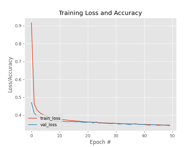 Figure 2: Here’s a plot of our training history. It shows little signs of overfitting, implying that our Keras and TensorFlow model is performing well on our OCR task. Figure 2: Here’s a plot of our training history. It shows little signs of overfitting, implying that our Keras and TensorFlow model is performing well on our OCR task.
As evidenced by the plot, there are few signs of overfitting, implying that our Keras and TensorFlow model is performing well at our basic OCR task. Let’s take a look at some sample output from our testing set: 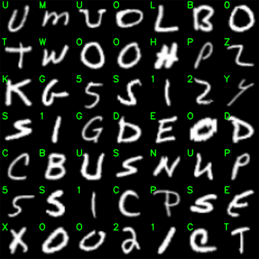 Figure 3: We can see from our sample output that our Keras and TensorFlow OCR model is performing quite well in identifying our character set. Figure 3: We can see from our sample output that our Keras and TensorFlow OCR model is performing quite well in identifying our character set.
As you can see, our Keras/TensorFlow OCR model is performing quite well! And finally, if you check your current working directory, you should find a new file named handwriting.model: $ ls *.model handwriting.modelThis file is is our serialized Keras and TensorFlow OCR model — we’ll be using it in next week’s tutorial on handwriting recognition. Applying our OCR model to handwriting recognition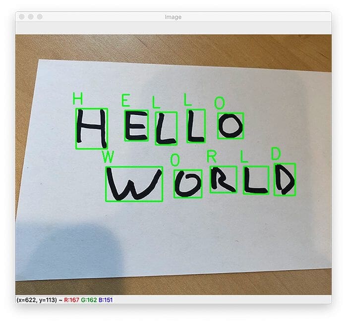 Figure 4: Next week, we will extend this tutorial to handwriting recognition. Figure 4: Next week, we will extend this tutorial to handwriting recognition.
At this point, you’re probably thinking: Hey Adrian, It’s pretty cool that we trained a Keras/TensorFlow OCR model — but what good does it do just sitting on my hard drive? How can I use it to make predictions and actually recognize handwriting? Rest assured, that very question will be addressed in next week’s tutorial — stay tuned; you won’t want to miss it! What's next? I recommend PyImageSearch University. Course information: 79 total classes • 101+ hours of on-demand code walkthrough videos • Last updated: August 2023 ★★★★★ 4.84 (128 Ratings) • 16,000+ Students EnrolledI strongly believe that if you had the right teacher you could master computer vision and deep learning. Do you think learning computer vision and deep learning has to be time-consuming, overwhelming, and complicated? Or has to involve complex mathematics and equations? Or requires a degree in computer science? That’s not the case. All you need to master computer vision and deep learning is for someone to explain things to you in simple, intuitive terms. And that’s exactly what I do. My mission is to change education and how complex Artificial Intelligence topics are taught. If you're serious about learning computer vision, your next stop should be PyImageSearch University, the most comprehensive computer vision, deep learning, and OpenCV course online today. Here you’ll learn how to successfully and confidently apply computer vision to your work, research, and projects. Join me in computer vision mastery. Inside PyImageSearch University you'll find: ✓ 79 courses on essential computer vision, deep learning, and OpenCV topics ✓ 79 Certificates of Completion ✓ 101+ hours of on-demand video ✓ Brand new courses released regularly, ensuring you can keep up with state-of-the-art techniques ✓ Pre-configured Jupyter Notebooks in Google Colab ✓ Run all code examples in your web browser — works on Windows, macOS, and Linux (no dev environment configuration required!) ✓ Access to centralized code repos for all 512+ tutorials on PyImageSearch ✓ Easy one-click downloads for code, datasets, pre-trained models, etc. ✓ Access on mobile, laptop, desktop, etc.Click here to join PyImageSearch University SummaryIn this tutorial, you learned how to train a custom OCR model using Keras and TensorFlow. Our model was trained to recognize alphanumeric characters including the digits 0-9 as well as the letters A-Z. Overall, our Keras and TensorFlow OCR model was able to obtain ~96% accuracy on our testing set. In next week’s tutorial, you’ll learn how to take our trained Keras/TensorFlow OCR model and use it for handwriting recognition on custom input images. To download the source code to this post (and be notified when future tutorials are published here on PyImageSearch), simply enter your email address in the form below!  Download the Source Code and FREE 17-page Resource Guide
Enter your email address below to get a .zip of the code and a FREE 17-page Resource Guide on Computer Vision, OpenCV, and Deep Learning. Inside you'll find my hand-picked tutorials, books, courses, and libraries to help you master CV and DL! |
 Course information:
79 total classes • 101+ hours of on-demand code walkthrough videos • Last updated: August 2023
★★★★★ 4.84 (128 Ratings) • 16,000+ Students Enrolled
Course information:
79 total classes • 101+ hours of on-demand code walkthrough videos • Last updated: August 2023
★★★★★ 4.84 (128 Ratings) • 16,000+ Students Enrolled
【本文地址】
| 今日新闻 |
| 推荐新闻 |
| 专题文章 |